
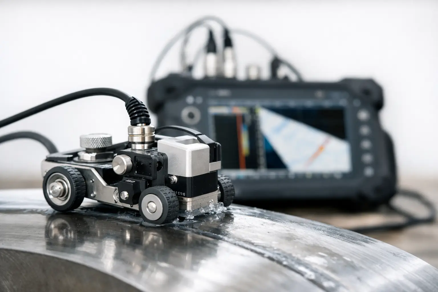

A PAUT image can look clean, repeatable and properly referenced, yet still be misleading if the encoder resolution is wrong. A scale error of only a few per cent can shift indications, distort weld geometry and make length sizing difficult to defend. Knowing how to set encoder resolution is therefore not just an instrument setup task. It is part of controlling the inspection.
The right setting depends on the scanner, encoder, wheel contact, scan plan and the smallest feature you need to represent. More resolution is not automatically better. Excessive sampling creates larger files, slows acquisition and can add no useful information. Too little sampling leaves gaps between A-scans and can hide the shape or true extent of an indication.
What encoder resolution actually controls
In encoded PAUT and ToFD, the encoder tells the instrument where each acquisition point sits along the scan. The instrument then builds a B-scan, C-scan or top view from those positions. Encoder resolution is commonly entered as distance per count, such as millimetres per pulse, although some instruments ask for pulses per millimetre or a total count over a known distance.
This is separate from the encoder's stated PPR, or pulses per revolution. PPR is a hardware specification. The value entered into the flaw detector or acquisition unit must reflect the real movement of the scanner on the component.
For a wheel encoder, the basic relationship is:
`distance per count = wheel circumference ÷ usable counts per revolution`
If a 100 mm circumference wheel has an encoder producing 1,000 usable counts per revolution, the theoretical resolution is 0.1 mm per count. But that is only the starting point. Some systems use quadrature decoding and count four transitions per encoder pulse, while others do not. Wheel compression, a dirty surface, poor contact and slip can all make the theoretical number wrong in practice.
The instrument must also know which encoder channel represents the scan axis and which represents index movement. Reversing direction is usually easy to correct in software. Assigning the wrong axis is less obvious and can produce a scan that appears valid until the image is reviewed against the weld layout.
How to set encoder resolution before a production scan
Start with the scan plan, not the encoder label. Establish the required scan-axis pitch, index pitch, scan length, coverage and expected scanning speed. Then configure the scanner and acquisition unit to achieve those values without exceeding the practical data rate.
1. Set the physical scanner correctly
Fit the correct encoder wheel or drive arrangement for the scanner and surface. A wheel that runs well on a smooth plate may slip on scaled pipe, uneven weld caps or a coated surface. Check that the wheel is loaded consistently and that the scanner is not rocking as it moves.
On modular scanner setups, make sure the encoder is coupled to the axis you intend to record. For a raster scan, the scan encoder usually tracks travel along the weld while the index encoder tracks movement across it. For a pipe scanner, the circumferential and axial axes need to match the reporting convention used for the job.
2. Enter a calculated starting value
Use the wheel circumference and the effective count per revolution to calculate a starting resolution. Confirm whether the acquisition software expects mm/count or counts/mm. These are inverses of each other, and entering one where the other is expected can produce an obvious but costly scaling error.
For example, if the wheel circumference is 200 mm and the system receives 2,000 counts per revolution, the starting value is 0.1 mm/count. If the software requests counts/mm, enter 10 counts/mm instead. Do not assume that a 500 PPR encoder gives 500 usable counts per revolution. Check the encoder and instrument documentation for the decoding method being used.
3. Calibrate against a measured distance
A calculated value should be verified on the actual scanner. Mark two points a known distance apart on a flat reference surface or use a calibrated scale fixed alongside the scan path. A distance of 500 mm or 1,000 mm is preferable to a short check because it exposes small errors more clearly.
Place the scanner at the first mark, zero the encoder position, then move to the second mark at a normal field scanning speed. Compare the displayed distance with the known distance. Repeat the movement in both directions. If the result changes depending on direction, investigate backlash, wheel slip, cable strain or a loose mechanical connection before adjusting a software factor.
Where the software allows a calibration routine, enter the known travel distance and let the instrument calculate the correction. Otherwise, use this relationship:
`new resolution = current resolution × known distance ÷ displayed distance`
If a 1,000 mm movement displays as 980 mm, multiply the current mm/count value by 1,000 ÷ 980. Recheck after the adjustment. The goal is repeatable travel measurement, not simply one pass that happens to land close to the mark.
4. Confirm the acquisition pitch
Encoder calibration tells the instrument the correct physical distance. Acquisition pitch determines how often data is captured along that distance. These settings are related but not interchangeable.
If the required scan resolution is 1.0 mm and the encoder calibration is 0.1 mm/count, set acquisition to record every 10 counts. If you want 0.5 mm sampling, acquire every five counts. Most PAUT instruments allow this to be entered directly as a scan resolution in millimetres, but understanding the count relationship helps when troubleshooting unexpected pitch values.
Select a pitch that suits the inspection
The correct scan pitch depends on beam coverage, focal spot size, inspection objective and the dimensions that need to be evaluated. For weld inspection, a practical starting point is to sample at a spacing finer than the effective beam width at the target area. This gives overlap between adjacent acquisition positions and avoids a striped or under-sampled image.
A 1.0 mm scan pitch may be suitable for a general weld volume assessment where the beam footprint and acceptance criteria support it. A 0.25 mm pitch may be justified when characterising small planar indications, examining a narrow region near the fusion face or producing detailed encoded records. It depends on the probe, wedge, material thickness and procedure requirements.
Index resolution requires the same thought. If adjacent raster lines are too far apart, coverage gaps can appear across the weld volume even when the scan-axis data is dense. If index steps are unnecessarily small, the scan takes longer and generates data that may not improve probability of detection.
For corrosion mapping, match the grid spacing to the expected corrosion morphology and the ultrasonic beam size. Broad general wall loss does not always need the same pitch as local pitting or erosion near a feature. Start with the inspection requirement, then set a grid that can represent the smallest relevant area without wasting site time.
Avoid the field issues that change resolution
Encoder calibration is not a set-and-forget number. A wheel encoder calibrated on a smooth calibration plate can behave differently on a hot, rusty or heavily coated component. The following checks are worth building into the pre-scan routine:
- Confirm the displayed travel over a known distance after changing wheels, scanner configuration or encoder mounting.
- Check for wheel slip at the normal scan speed, especially on pipe, curved surfaces and rough weld caps.
- Verify scan and index directions with a short encoded test run before collecting production data.
- Watch the live position readout for dropped counts or erratic movement caused by damaged cables or poor connectors.
This takes minutes and prevents a longer discussion later about whether the encoded position can be trusted.
Resolution, speed and file size are a trade-off
It is tempting to set the finest available resolution and treat it as a safer option. In field work, that approach can create problems. A fine pitch multiplies the number of A-scans, increases file size and can force a slower scanner speed to keep the acquisition unit within its encoder-triggered data rate. If scanning speed exceeds what the system can capture, data may be skipped, position tracking may become unreliable or the instrument may warn of lost data.
Calculate the likely acquisition rate before starting. A scan speed of 100 mm/s at 0.5 mm pitch requires 200 acquisitions per second on that axis. At 0.1 mm pitch, the same movement requires 1,000 acquisitions per second. Add the selected focal laws, A-scan length and index movement, and the practical system limit can be reached quickly.
Choose the coarsest pitch that still meets the procedure and inspection objective. That is not cutting corners. It is matching the data density to the defect detection and sizing task. PAUT.Tech equipment is designed around this kind of fit-for-purpose setup: a scanner should support the job without turning a straightforward inspection into a complicated rebuild or an oversized data collection exercise.
When the image does not match the component
A distorted encoded image is often blamed on the probe setup first, but encoder settings deserve an early check. If a known 100 mm feature measures 95 mm or 105 mm in the scan, recalibrate distance. If the image is stretched only in one direction, check the corresponding encoder axis and acquisition pitch. If the image shows intermittent bands, look for lost counts, poor wheel contact or scan speed that is too high for the selected resolution.
Also check whether the scanner has moved relative to the weld centreline. An encoder can report distance perfectly while the scanner itself wanders. Good encoded data needs accurate position measurement and controlled mechanical tracking.
Before collecting the final scan, run a short encoded pass over a known reference, confirm scale and direction, then review the pitch and coverage on the live display. That small check is usually the quickest way to ensure the recorded image represents what is actually in front of the probe.