A useful corrosion job hardware example is not a catalogue of components. It is a scanner arrangement that gets reliable thickness data across a corroded surface without consuming half the shift in setup, adjustment and repeat runs. For a technician working on ageing pipework or a vessel shell, the hardware has to stay coupled, maintain positional accuracy and cope with the real condition of the surface.

Consider an external corrosion mapping job on a carbon-steel process line. The objective is to create an encoded thickness map over a 1.2 metre length of pipe, identify localised wall loss, and provide data that can be reviewed against the client’s minimum remaining wall requirements. This is where task-specific scanner hardware makes more sense than rebuilding a general-purpose scanner from scratch.

The corrosion job hardware example

For this example, assume a 450 mm outside diameter pipe with an original nominal wall thickness of 8 mm. The inspection area is externally accessible after coating removal, but the surface still has typical plant-condition issues: light pitting, minor weld spatter near attachments, uneven preparation and restricted clearance on one side of the line.

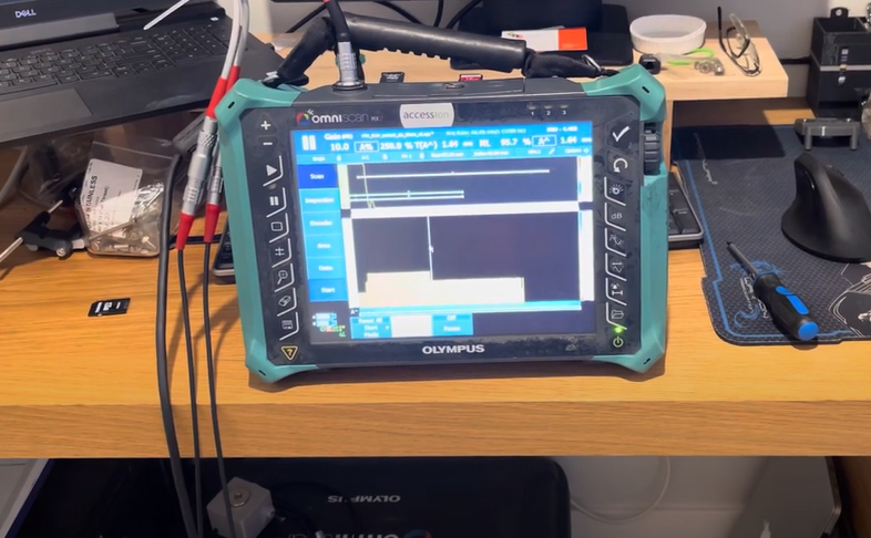
The inspection setup consists of an encoded pipe scanner fitted with a phased array probe, a suitable zero-degree wedge, a compact encoder and a data acquisition instrument capable of recording encoded A-scan data. The scanner is configured to travel around the circumference while the probe indexes along the pipe axis. That produces a raster coverage pattern, allowing the operator to generate a thickness map rather than relying on isolated spot readings.

The exact hardware changes with pipe diameter, surface condition and access. The principle does not: the scanner controls probe position, the encoder records it, and the probe configuration produces enough resolution to identify the wall-loss mechanism that matters.

Scanner choice comes before probe choice

A common mistake is selecting the probe first and then trying to make a scanner fit around it. On a corrosion job, scanner geometry should be decided from the component and access constraints.

For a pipe in open access, a purpose-built pipe scanner that follows the pipe circumference is usually the efficient choice. It gives repeatable circumferential travel and can be indexed along the axial direction in controlled increments. For a large-diameter vessel or a flat plate, a magnetic wheel scanner or encoded raster scanner may be the better arrangement.

The key question is whether the scanner can maintain stable contact and consistent tracking over the full inspection area. A lightweight scanner is useful when working overhead or from rope access, but it still needs enough stiffness that the probe does not wander as it crosses a local depression or rough patch. Too much compliance can blur the map. Too little compliance can cause coupling loss on an uneven surface.

A modular arrangement is valuable here. A technician may need one scanner set up for a 450 mm pipe and another ready for a vessel patch job later that day. Keeping dedicated hardware available avoids stripping down the corrosion scanner every time a different inspection arrives.

Probe and wedge selection for the wall range

For an 8 mm carbon-steel pipe with general and localised corrosion, a 5 MHz linear array is often a sensible starting point. It can provide good near-surface resolution and a sufficiently small sampling footprint for practical corrosion mapping. However, it is not a universal answer.

A lower-frequency probe may be more appropriate where the material is coarse-grained, heavily attenuating or substantially thicker. A higher-frequency option can improve resolution on thinner, smoother material, but may become less forgiving on rough surfaces or through coating residue. The right selection depends on signal quality from representative sound material, not the number printed on the probe case.

For standard thickness mapping, a zero-degree wedge is generally used to direct sound through the wall. The wedge needs to suit the component curvature and probe dimensions. A poor curvature match creates inconsistent coupling pressure and variation in the water path or delay, which can appear as false thickness variation if the setup is not properly calibrated.

Before mapping begins, confirm the measurement method against known thickness. Use a sound reference area, check repeatability at several positions, and make sure the gate captures the correct backwall response. If corrosion is severe enough to create multiple reflections, rough backwall echo behaviour or difficult-to-separate signals, the inspection procedure may need a different analysis approach rather than simply tighter gates.

Encoding is what turns readings into defensible coverage

A hand-held ultrasonic thickness gauge remains useful for quick checks and follow-up verification. It does not replace encoded coverage when the client needs to understand the distribution and extent of corrosion.

In this example, the circumferential encoder records scanner travel while the axial index is controlled in set increments. The index increment should be selected from the required map resolution and expected defect morphology. For broad general thinning, a larger increment may be adequate. For pitting or narrow channels of wall loss, a tighter index is needed so the feature is not missed between scan lines.

There is a trade-off. Tighter resolution increases scan time, data volume and the chance that a rushed operator loses discipline around couplant, cable management or surface changes. A 1 mm by 1 mm grid may be justified on a small critical area, while a wider grid can be more practical for screening a large low-risk section. The inspection plan should state the coverage and sampling rationale before arriving on site.

Encoder resolution also needs to match the job. There is little value in a fine-resolution encoder if the scanner wheels slip or the chain is loose enough to shift position during travel. Check the mechanical drive, establish a clear scan origin and confirm that the displayed distance agrees with a physical reference. This basic check prevents a surprising number of reporting problems.

Field setup details that affect the result

The hardware configuration only works when the job is prepared properly. Start by marking the inspection boundary, pipe orientation and scan datum. On a pipe, use a consistent reference such as the 12 o’clock position and record the direction of travel. That makes later data review and repeat inspection far easier.

Surface preparation should be proportionate to the required accuracy. Loose scale, sharp weld spatter and damaged coating can obstruct the scanner or destabilise coupling. The aim is not to make the component look new. It is to create a traversable, couplant-compatible surface where the probe can produce repeatable signals.

Couplant delivery deserves attention. A manually applied couplant bead can be adequate for a short, accessible scan. On a longer raster job, an integrated reservoir or controlled feed reduces interruptions and helps maintain signal consistency. Excess couplant is not a cure for poor scanner fit, though. If the scanner rocks, tracks inconsistently or applies uneven pressure, more couplant only masks the mechanical issue for a short distance.

Keep instrument and probe cables secured so they cannot drag on the scanner. On a pipe rack, a cable catching on a support or sharp edge can alter the scanner path without the operator immediately noticing. A simple strain-relief point and a clear cable route are practical controls, particularly when scanning from a platform or in a congested plant area.

A workable scan sequence

With the scanner fitted and the probe aligned, perform a short trial run over sound wall. Review the A-scan response, thickness stability and encoder count before committing to the full raster. Then scan one or two complete lines and inspect the developing map. If there are blank areas, unexpected striping or a repeating thickness offset, stop and correct the cause early.

For the 1.2 metre pipe section in this example, the operator can complete a controlled circumferential pass, index the scanner along the axis, and repeat until the planned coverage is achieved. At intervals, verify the result with local manual readings in sound material and at selected low-thickness indications. This is not because encoded PAUT is unreliable. It is a sensible check that confirms the setup remains stable as site conditions change.

After scanning, identify the lowest measured areas, assess the shape and spread of wall loss, and retain the encoded data with the scan plan and calibration evidence. A colour thickness map is useful, but the underlying A-scans and position data are what allow another competent reviewer to assess the call.

Where purpose-built hardware saves time

The practical benefit of this corrosion job hardware example is not that every component is specialised for one pipe size forever. It is that the scanner, encoder mounts, probe holders and wedges are selected to work together for the inspection task.

PAUT.Tech hardware is built around this approach: practical scanner assemblies that can be allocated to corrosion work instead of repeatedly dismantling a premium weld scanner for a different job. For a small NDT business, that can mean one technician maps corrosion while another keeps a weld scanner prepared for production inspection.

The best corrosion setup is the one that produces repeatable, traceable data without asking the operator to fight the hardware. Start with the component geometry and coverage requirement, then build the scanner arrangement around the job. That decision usually pays back before the first scan line is complete.