
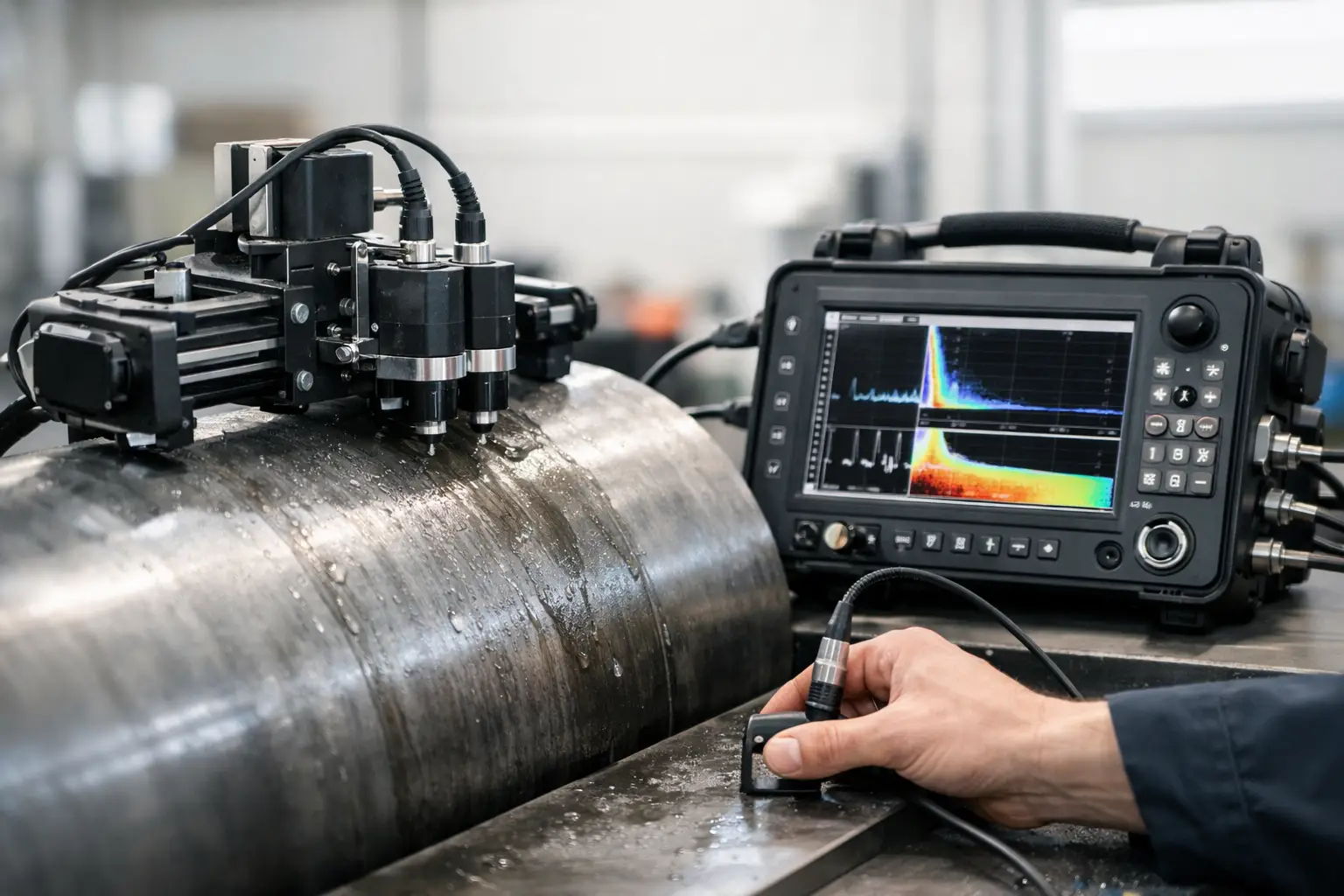

A bad ultrasonic thickness scanner setup rarely announces itself at the first scan line. It shows up later as a questionable thin spot, a map that will not line up with the component, or repeat readings that change when the operator returns for a second pass. For corrosion mapping work, the scanner, probe, encoder and instrument need to operate as one measurement system.
The aim is not simply to collect lots of A-scans. It is to produce thickness data that can be located, repeated and defended. That means setting the job up around the material condition, scan area, required resolution and reporting decision before putting a probe in the scanner.
Start with the inspection decision
Thickness mapping is often requested as though it is a single task, but the setup changes depending on what the client needs to know. A broad screening survey of a vessel shell does not need the same point density as a local corrosion assessment around a nozzle, patch repair or suspected under-insulation corrosion area.
Define the scan boundary, direction of travel, grid spacing and acceptance criteria first. Confirm whether the report must show minimum remaining wall, localised pitting, average loss, or a map suitable for engineering assessment. These choices drive probe selection, scanner travel and encoder resolution.
It also pays to establish where the datum will sit on the component. A physical reference such as a weld toe, plate edge or clearly marked centreline makes a follow-up inspection much more useful. If the scanner is started from an arbitrary point each time, comparing maps between shutdowns becomes unnecessarily difficult.
Match the probe to the condition, not the catalogue
A dual-element probe is often the practical choice for corrosion mapping on steel because it performs well on moderately rough surfaces and helps separate the initial pulse from the backwall response. Probe frequency and element size, however, still depend on the job.
Higher frequencies can improve near-surface resolution on clean material with fine corrosion. They can also lose penetration when the surface is coarse, the material is attenuative, or the remaining wall is substantial. A lower-frequency probe may provide a more stable backwall signal through coatings or rough service-aged steel, but it can be less effective for resolving small, sharp pits.
Do not assume a coating is harmless just because the instrument produces a number. A sound coating may be included in the measured path if the setup has not been configured to account for it. If coating thickness matters, establish whether it will be removed in the scan band, compensated for in the instrument, or treated as part of the reported result. The correct approach depends on the procedure, component history and required accuracy.
Probe wear is another field issue. A worn face, damaged membrane or inconsistent delay line can shift readings across a long scan. Inspect the probe before calibration, not after the map has been collected.
Use a scanner that holds the probe consistently
A scanner does more than provide a handle for the probe. It controls probe pressure, travel direction and positional data. If the probe rocks as it crosses a weld cap, scale edge or curved surface, the coupling and sound path can change enough to create false variation in the map.
Set the scanner so the probe is supported without excessive force. Too little contact pressure risks intermittent coupling. Too much pressure can squeeze couplant away, accelerate wear and make the operator fight the scan. On curved surfaces, use a frame or shoe arrangement that matches the radius as closely as practical. A scanner that tracks straight on plate may not maintain probe alignment around a small-bore pipe.
For repeated work, a purpose-built setup usually saves more time than continually rebuilding a general-purpose scanner. The saving is not only assembly time. It is the reduction in adjustment, checking and operator variation before each job.
Configure encoding before collecting data
An encoded thickness map is only as useful as its position data. Confirm the scan axis, index axis, scan length and index increment in the instrument before starting. Then verify the direction shown on screen matches the scanner movement. Reversed encoding is easy to correct before a job and awkward to explain once the scan has been reported.
Encoder calibration should be checked against a measured travel distance on the actual scanner arrangement. Mark a known length on the component or a flat reference surface, move the scanner across it, and compare the reported distance. A wheel that slips on dusty steel or rides over uneven coating can introduce positional error even when the encoder itself is configured correctly.
The right resolution is a trade-off. Very fine indexing can create a detailed map, but it increases scan time, file size and the chance that operators rush the travel to get through the area. Excessively coarse indexing can miss isolated pitting. Select a pitch that is appropriate for the smallest feature the inspection is expected to identify, then use a travel speed that allows stable acquisition.
Calibrate for the material and confirm the gate
Velocity, zero offset, range and gate placement need to suit the probe and the expected thickness range. A two-point calibration on suitable reference steps remains the practical starting point where procedure permits. Use calibration material with a known thickness and, ideally, similar acoustic properties to the component being examined.
Calibration is not complete because the instrument displays the reference thickness correctly once. Check the response at more than one point, especially near the minimum and maximum wall values expected in the scan. If the job involves thin remaining wall beside much thicker parent material, make sure the gate and range allow both conditions to be measured without ambiguity.
Review the A-scan while setting the gate. Automatic thickness measurement can be quick, but it cannot judge whether it is tracking the correct echo in every condition. On corroded material, multiple echoes, mode-converted signals and noisy backwalls can appear. The selected gate should follow the true backwall response, not a convenient earlier indication.
Where the instrument supports amplitude monitoring or A-scan storage, use it sensibly. It can help identify low-coupling areas and support later review. It does not replace watching signal quality during the scan.
Treat coupling as part of the measurement system
Couplant choice and application matter more than they seem. Use a couplant that remains workable at the component temperature and will not run out of the scan path immediately. On vertical surfaces, a thicker gel may be preferable. On hot surfaces, confirm the temperature rating of both couplant and probe before beginning work.
Prepare the surface enough to obtain consistent contact. This does not always mean grinding a large clean patch. It means removing loose scale, dirt, overspray and material that causes the probe to skip or the wheel to slip. Any surface preparation should be recorded where it could affect coating condition or client requirements.
During the first scan line, watch for signal drop-out, sudden thickness steps that do not match the A-scan, and changes as the scanner crosses a surface feature. Stop and investigate rather than assuming software filtering will fix the map later. Filtering can make a report look cleaner while hiding a setup problem.
Validate the scan before leaving the job
A practical check is to scan a short section twice, preferably in opposite directions where the setup allows. The map should reproduce the same general profile and minimum areas within the tolerance defined by the inspection procedure. If it does not, investigate calibration, encoder slip, coupling, probe contact and operator technique.
Confirm selected low-thickness areas manually with a conventional spot reading or an independent pass. This is especially useful for isolated minima that may drive repair or remaining-life decisions. A colour map is persuasive, but the A-scan and repeat measurement are what give the indication credibility.
Before packing down, save the raw data, setup file, calibration record and component reference details. Record the probe model, frequency, scanner configuration, scan pitch, gain, velocity and any coating treatment. These details turn a one-off survey into baseline data that another technician can repeat.
Build setups around real field constraints
The best arrangement is rarely the most elaborate one. It is the one that fits the available access, component geometry, required coverage and time on site without compromising data quality. A compact manually indexed scanner can be the sensible answer for a small local assessment. A longer encoded frame may be justified when a large area needs consistent, reportable coverage.
This is where modular hardware earns its place. Keeping dedicated or quickly configured scanner arrangements for plate corrosion, pipe work and local repairs reduces the pressure to force one expensive system into every task. PAUT.Tech designs its scanner hardware around that practical reality: equipment should suit the job, not create another job before inspection can begin.
A disciplined setup takes a little longer before the first line is scanned. It saves far more time than returning to site because a map cannot be trusted. When the probe response, scanner travel and positional data agree, the thickness map becomes a decision-making tool rather than a colourful picture.